En pocas palabras
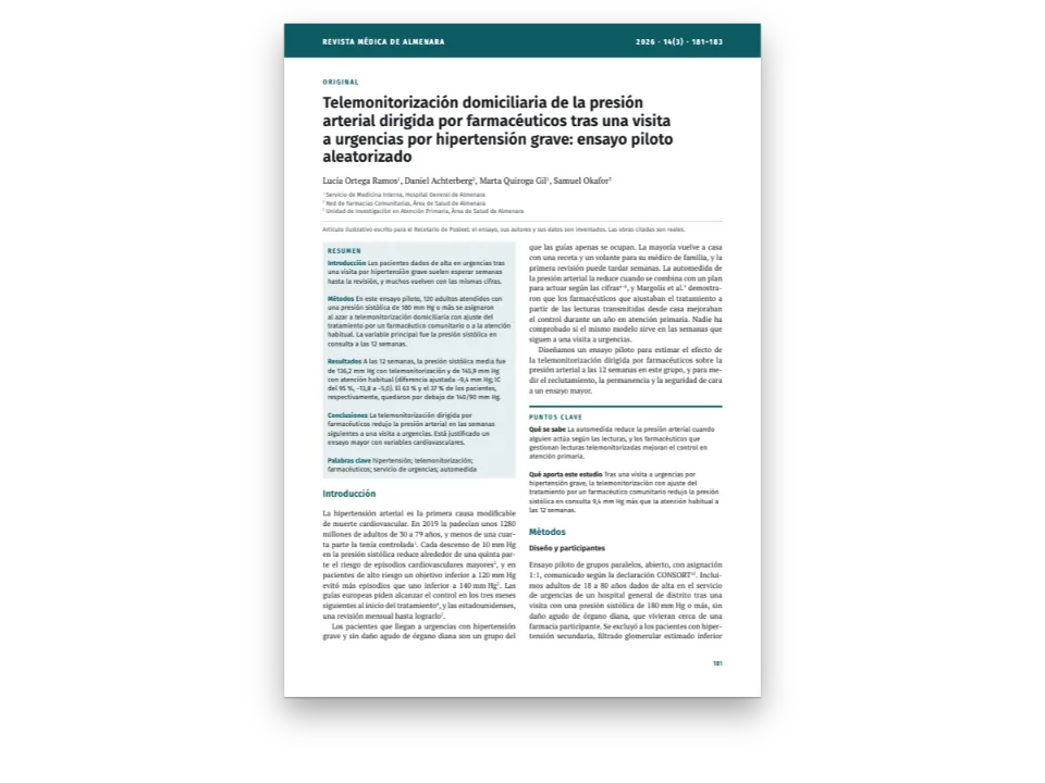
Un artículo de biología muy citado, abreviado y compuesto de nuevo como en una revista. Los Métodos van después del texto, en letra más pequeña, y sus referencias siguen contando desde donde lo dejó el texto principal.
Lo que vas a componer
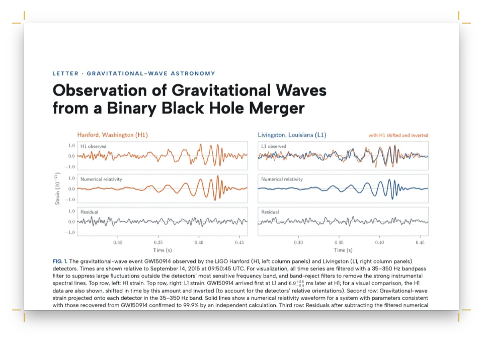
Cinco páginas de un artículo de revista de ciencias de la vida en A4: Highly accurate protein structure prediction with AlphaFold, de Jumper y colaboradores, abreviado a partir de Nature con licencia CC BY 4.0. Una banda azul abre la primera página sobre el título, los 34 autores en 7,4 pt con los números de filiación volados y el resumen en negrita a todo el ancho. Debajo, a todo el ancho, va la figura 1: un gráfico de barras con las precisiones de CASP14 que cita el texto y el esqueleto de la diana T1049 trazado desde el PDB, con el modelo de AlphaFold dibujado dentro y coloreado según su confianza. El texto cita con los números volados de Nature. El texto principal se cierra con las referencias 1–35. Los Métodos siguen en 8,2 pt, y una obra que citan por primera vez toma el número siguiente, así que su propia lista empieza en el 36, como en la revista.
Esta receta responde a
- ¿Cómo compongo la sección de Métodos de un artículo en un cuerpo menor después del texto principal, con sus citas continuando la numeración?
- ¿Cómo vuelvo a componer con Postext un artículo de acceso abierto de arXiv o PubMed Central, con sus citas, sus figuras y su línea de licencia?
- ¿Cómo pongo los números de cita en superíndice y hago que los DOI sean enlaces, como en las revistas médicas?
- ¿Cómo añado una figura con pie numerado y la cito en el texto («véase la fig. 3.2»)?
La respuesta corta
// [@key] prints a raised number in order of first citation, so a work the Methods cite for
// the first time takes the next number after the main text's last, and one cited again
// keeps its number. Nature prints two lists, and :::bibliography{scope=new} lists only the
// works no earlier list printed: the same block after the main text and after the Methods
// sets references 1–35, then 36–55.
registerCitationEngine(createCiteprocEngine({ styles: STYLES, locales: LOCALES }));
const citations = {
  style: 'nature', // raised 1–4, "Nature 577, 706–710 (2020)." entries
  bibliography: { fontSize: em(0.8), lineHeight: pt(9.6), entrySpacing: pt(0.8),
    labelWidth: mm(5), labelAlign: 'right' }, // 9. and 10. end together
};
const references = '### References\n\n:::bibliography{title="" scope=new}';
// "# Methods {style=\"methods\"}" opens a section that runs to the end of the article: an H1
// that breaks nothing, names no running chapter and sets its body two sizes down.
const methods = { id: 'methods', numbered: false, runningChapter: false,
  breakBefore: { enabled: false }, fontFamily: SANS, fontSize: pt(11.5), lineHeight: pt(LEAD),
  fontWeight: 700, color: col('ink'), marginTop: pt(LEAD), marginBottom: pt(LEAD / 2),
  bodyStyle: { fontSize: pt(8.2), lineHeight: pt(SMALL) } };
Ingredientes
- Funciones
- Estilos de títuloCitas en un estilo de citaBibliografía a partir de las referenciasSuperíndices y subíndicesAperturas diseñadasAtributos de títuloRecuadrosRecuadros a todo el anchoCabeceras y foliosCabeceras según el tipo de páginaFiguras justo aquíEstilo de los piesLíneas de fuente y créditoEstilo de tablasPies numeradosEstilos de párrafoPaleta de color semánticaExportación a PDFFuentes incrustadas en el PDF
- También usa
- Citas que colocan las figurasFigura y Tabla en tu idiomaTipos de recurso propiosFiguras y tablas como recursosCapítulos sin número
- Tipografía
- Noto Serif, Noto Sans (SIL OFL 1.1)
- Recursos
- Figura 1b, coordenadas Cα experimentales de PDB 6Y4F (Jiang et al. 2020), dibujadas en código (Worldwide Protein Data Bank, CC0 1.0)
- Figura 1b, modelo AF-B4EUK6-F1 de AlphaFold DB (AlphaFold Monomer v2.0) y su pLDDT, superpuesto y dibujado en código (DeepMind Technologies Limited and EMBL-EBI, AlphaFold Protein Structure Database, CC BY 4.0)
Elaboración
#1 · Dos listas de referencias y una sola numeración
El código es la respuesta corta de arriba. Las citas se numeran por orden de primera aparición, así que no hay que hacer nada para seguir la cuenta: jackhmmer, que se cita por primera vez en los Métodos, recibe el 36, mientras que el campo de fuerzas Amber, citado antes en el texto, conserva su 30. Las listas salen de :::bibliography{scope=new}, que imprime solo las obras que ninguna lista anterior ha impreso. El script pone el mismo bloque tras la Discusión y tras los Métodos: el primero compone de la 1 a la 35, el segundo de la 36 a la 55, y Amber no se repite. El título de los Métodos es un encabezado de primer nivel con estilo propio; su bodyStyle compone la sección en 8,2 pt sobre 10,8 pt, breakBefore: { enabled: false } lo deja en la columna y runningChapter: false mantiene en las cabeceras el título del artículo. Para tu propio artículo, pega la exportación de tu .bib en un bloque :::references{format=bibtex}, cita con [@clave] pegado a la palabra y cambia nature por el estilo de tu revista.
#2 · Un bloque de título para 34 autores
const text = (id, content, family, size, extra) => ({ kind: 'text', id, content, align: 'left',
  fontFamily: family, fontSize: pt(size), color: col('ink'), overflow: 'wrap', ...extra });
const at = (to, edge, x, y, width) => ({ anchor: { to, edge }, offset: { x: mm(x), y: mm(y) },
  ...(width && { size: { width: mm(width), height: 'auto' } }) });
const caps = { fontFamily: SANS, fontWeight: 600, letterSpacing: pt(1.4),
  textTransform: 'uppercase' };
const titleBlock = { enabled: true,
  minHeight: mm(50),
  slot: { elements: [
    { kind: 'box', id: 'band', style: { backgroundColor: col('accent') },
      placement: { anchor: { to: 'page', edge: 'top-left' },
        size: { width: 'fill', height: mm(14) } } },
    text('kicker', '{attr.kicker}', SANS, 8.5, { ...caps, color: col('paper'),
      placement: at('page', 'top-left', INNER, 5.6, 120) }),
    text('title', '{titleText}', SANS, 23, { fontWeight: 700, lineHeight: 1.12,
      placement: at('container', 'top-left', 0, 1, MEASURE - 30) }),
    text('authors', '{attr.authors}', SANS, 7.4, { inlineMarks: true, lineHeight: 1.42,
      placement: at('#title', 'below', 0, 4, MEASURE) }),
    { kind: 'rule', id: 'rule', thickness: pt(0.5), color: col('rule'),
      placement: at('#authors', 'below', 0, 3, MEASURE) },
    text('source', '{attr.source}', SANS, 7, { color: col('muted'),
      placement: at('#rule', 'below', 0, 1.6, MEASURE) }),
  ] },
};
La lista de autores es un solo atributo del encabezado, authors="John Jumper^1,4^, Richard Evans^1,4^, …", compuesto en Noto Sans de 7,4 pt a toda la medida, donde los 34 nombres ocupan cinco líneas. inlineMarks sube los números de filiación. Las filiaciones y la nota de contribución igual van al final, en Author information, como las imprime Nature, y así la primera página conserva sitio para el resumen y la figura. No se omite ningún autor: la cabecera de las páginas pares abrevia la lista a Jumper et al.
#3 · El resumen a todo el ancho y la figura 1 debajo
const resources = () => [
  { id: 'fig1', typeId: 'figure', kind: 'svg', createdAt: 0, updatedAt: 0,
    placement: { position: 'here', span: 'page' },
    svg: { fileId: 'fig1.svg', width: 1780, height: 640 },
    caption: '**AlphaFold produces highly accurate structures.** **a**, Median accuracy on the '
      + 'CASP14 domains of AlphaFold and of the next best method, as r.m.s.d.~95~ over Cα atoms '
      + '(backbone) and over all atoms, with 95% confidence intervals; the dashed line is the '
      + 'width of a carbon atom, about 1.4 Å. **b**, CASP14 target T1049 (PDB 6Y4F): the '
      + 'experimental Cα trace (grey) and the AlphaFold model of the same chain, coloured by '
      + 'its per-residue confidence (pLDDT).',
    note: 'Redrawn for this edition. a, from the values given in the text (the original plots '
      + 'the top 15 of 146 entries). b, from PDB 6Y4F (CC0) and AlphaFold DB model '
      + 'AF-B4EUK6-F1, AlphaFold Monomer v2.0 (CC BY 4.0), superposed on 134 Cα atoms; the '
      + 'original shows the CASP14 prediction.',
    altText: 'Bars: AlphaFold 0.96 and 1.5 Å, next best 2.8 and 3.5 Å. Two backbones that '
      + 'lie almost on top of each other.' },
  { id: 'tbl-timings', typeId: 'table', kind: 'table', createdAt: 0, updatedAt: 0,
    placement: { position: 'here' },
    caption: '**Inference times.** One model on one V100 GPU, by protein length.',
    note: 'Compiled for this edition from the timings given in ‘Inference regimen’.',
    table: { model: { headerRowCount: 1, columnWidths: [1, 1.3, 1.3], rows: [
      ['Residues', 'With ensembling (CASP14)', 'Without ensembling'],
      ['256', '4.8 min', '0.6 min'], ['384', '9.2 min', '1.1 min'],
      ['2,500', '18 h', '2.1 h'],
    ].map((row, r) => row.map((content, c) => ({ content, ...(r === 0 && { isHeader: true }),
      ...(c > 0 && { align: 'right' }) }))) } } },
];
El resumen es un recuadro con span: 'page' y sin borde, con el texto en Noto Sans seminegrita. La figura 1 lo sigue como ::resource{id="fig1"}, y su colocación, { position: 'here', span: 'page' }, la compone sobre las dos columnas en ese punto; las dos columnas de texto empiezan bajo su pie. El pie empieza con una frase en negrita, como los de Nature; el captionPrefix del tipo y el labelSeparator del estilo de pie hacen que la etiqueta diga Fig. 1 |. La tabla 1 va incrustada donde está, en los Métodos, con position: 'here', y se queda en su columna.
#4 · El esqueleto de una proteína a partir de coordenadas abiertas
// PDB 6Y4F chain A, residues 25–158: Cα x, y in tenths of Å, depth z in Å (CC0)
const EXP = [
  -56,-91,-6,-36,-77,-3,-4,-98,-2,26,-81,-1,63,-86,-1,95,-73,1,116,-100,2,146,
  -79,3,159,-46,2,187,-34,4,209,-6,3,211,10,0,187,17,-3,182,53,-2,185,46,2,
  167,14,3,148,-4,6,122,-28,4,109,-58,6,76,-67,4,45,-89,4,11,-79,3,-2,-114,
  3,-37,-116,1,-64,-95,0,-87,-117,-2,-124,-110,-2,-135,-80,-5,-161,-95,-7,-158,
  -74,-10,-173,-41,-9,-141,-20,-9,-148,15,-8,-128,31,-5,-105,55,-7,-106,82,-4,
  -144,80,-3,-156,116,-3,-122,132,-2,-126,155,1,-102,131,3,-88,98,2,-68,72,4,
  -58,37,3,-23,33,4,6,10,5,32,28,2,59,21,0,68,31,-4,89,62,-3,96,70,-7,102,
  52,-10,65,59,-11,53,41,-8,39,71,-6,38,70,-2,64,79,0,59,86,4,33,60,5,42,
  36,8,7,42,9,-29,48,8,-55,21,9,-88,39,8,-105,69,6,-122,57,3,-134,87,1,-170,
  78,2,-167,42,1,-180,38,-3,-165,5,-4,-132,-13,-3,-150,-42,-2,-161,-18,1,-125,
  -6,1,-114,-43,2,-141,-49,4,-129,-20,6,-92,-30,6,-98,-66,7,-120,-57,10,-94,
  -33,11,-62,-52,11,-54,-89,11,-36,-104,8,-8,-109,7,3,-73,8,40,-75,9,67,-51,
  10,93,-26,9,92,8,7,119,30,5,128,47,2,151,77,2,149,93,-2,152,82,-5,173,52,
  -6,150,22,-6,162,-13,-8,144,-44,-6,119,-43,-9,109,-8,-8,106,-15,-4,72,-24,
  -3,53,-20,0,15,-23,0,-19,-8,1,-20,28,-1,-48,53,-1,-38,89,0,-52,122,1,-25,
  128,3,-19,107,7,18,115,7,47,129,5,57,121,1,26,112,-1,28,122,-4,-9,117,-5,
  -8,83,-3,-9,51,-5,-13,14,-5,-49,3,-4,-61,-14,-8,-50,-50,-8,-19,-46,-6,8,
  -72,-7,43,-65,-6,67,-94,-5,43,-121,-6,32,-148,-3,-6,-157,-3,-17,-192,-4,-23,
  -216,-1,
];
// AlphaFold DB AF-B4EUK6-F1, the same residues superposed on 6Y4F (CC BY 4.0)
const MODEL = [
  -57,-93,-6,-37,-77,-3,-5,-98,-2,25,-82,-1,63,-87,-1,94,-74,1,112,-103,3,144,
  -84,3,158,-50,2,189,-34,4,209,-2,3,212,16,0,187,21,-3,181,57,-2,181,48,2,
  166,13,2,148,-4,5,122,-29,4,110,-58,6,76,-66,4,46,-88,4,12,-79,3,0,-115,3,
  -37,-113,2,-64,-95,0,-87,-118,-2,-125,-110,-2,-136,-81,-4,-162,-95,-7,-155,
  -74,-10,-173,-42,-9,-141,-22,-9,-146,14,-8,-126,31,-5,-102,55,-7,-106,83,-4,
  -143,81,-4,-156,117,-3,-122,132,-2,-123,157,1,-101,132,3,-86,98,2,-68,72,4,
  -58,36,3,-22,32,4,7,8,4,32,26,2,61,20,0,67,31,-4,89,62,-3,95,73,-7,100,
  56,-10,64,67,-11,52,44,-8,40,74,-6,38,68,-2,65,77,0,59,84,4,35,56,5,45,
  30,8,10,37,9,-25,47,8,-54,21,9,-86,40,8,-105,69,6,-120,56,3,-132,87,1,
  -169,78,2,-166,42,0,-177,37,-3,-163,3,-4,-130,-15,-3,-150,-42,-2,-162,-17,1,
  -125,-5,1,-114,-42,2,-142,-47,5,-129,-15,7,-93,-28,6,-103,-62,8,-122,-46,11,
  -90,-26,12,-62,-52,11,-59,-89,10,-37,-104,7,-8,-110,7,3,-74,8,40,-74,9,66,
  -48,10,95,-26,9,95,7,7,124,30,6,127,45,2,147,78,2,145,92,-1,153,87,-5,172,
  54,-6,147,26,-7,158,-6,-8,145,-39,-7,117,-42,-10,105,-7,-8,106,-14,-5,72,
  -24,-3,54,-21,0,16,-25,0,-18,-8,0,-19,27,-1,-48,52,-1,-37,88,0,-51,122,1,
  -26,127,4,-23,104,7,15,108,7,45,124,5,57,120,2,26,111,-1,31,123,-4,-7,116,
  -5,-5,83,-3,-8,51,-5,-12,14,-5,-48,2,-5,-62,-14,-8,-53,-52,-8,-20,-47,-6,5,
  -74,-7,39,-66,-5,64,-95,-5,99,-89,-7,117,-72,-4,146,-94,-2,178,-75,-3,190,
  -46,-1,
];
// The model's per-residue pLDDT, read from its B-factor column
const PLDDT = [
  87,89,87,87,83,87,82,84,85,84,82,79,81,86,90,89,93,93,94,95,92,95,87,90,
  93,87,89,88,82,75,87,92,97,98,98,98,98,98,98,98,98,99,99,99,99,99,98,96,
  94,93,90,84,87,89,95,95,96,97,98,98,98,98,98,98,99,99,99,98,98,98,98,97,
  97,98,98,98,98,98,98,97,98,98,96,95,89,96,97,96,96,96,96,94,93,91,88,86,
  82,73,67,61,61,69,83,89,96,97,98,99,99,98,98,97,96,97,96,96,95,95,96,97,
  97,96,97,94,87,90,84,82,69,65,64,61,55,53,
];
const n2 = (v) => +v.toFixed(2);
// The figure names Noto Sans on its root; loadSvg embeds the faces its labels set
// (inlineSvgFonts), so the canvas and the PDF draw them in the page's own sans.
const label = (x, y, s, size = 2.5, extra = '') => { // ink unless extra sets a fill
  const fill = extra.includes('fill') ? '' : `fill="${palette.ink}" `;
  return `<text x="${n2(x)}" y="${n2(y)}" font-size="${size}" ${fill}${extra}>${s}</text>`;
};
// a: median r.m.s.d.95 with its 95% interval, as the text gives them
const ACCURACY = [
  { group: 'Backbone', af: [0.96, 0.85, 1.16], next: [2.8, 2.7, 4.0] },
  { group: 'All-atom', af: [1.5, 1.2, 1.6], next: [3.5, 3.1, 4.2] },
];
function bars() {
  const [L, B, T, H] = [9, 54, 8, 4.5]; // axis left, baseline, top, Å at the top
  const y = (v) => B - (v / H) * (B - T);
  let s = label(0, 3.2, 'a', 3.6, 'font-weight="700"');
  for (const v of [0, 1, 2, 3, 4]) {
    s += `<path d="M${L} ${n2(y(v))}H58" stroke="${palette.rule}" stroke-width="0.15"/>`
      + label(L - 1.5, y(v) + 0.9, v, 2.5, 'text-anchor="end"');
  }
  s += label(1.6, 31, 'r.m.s.d.<tspan font-size="1.8" dy="0.6">95</tspan><tspan dy="-0.6"> (Å)'
    + '</tspan>', 2.5, 'text-anchor="middle" transform="rotate(-90 1.6 31)"');
  ACCURACY.forEach(({ group, af, next }, g) => {
    const x0 = L + 4 + g * 24;
    [[af, palette.accent], [next, palette.rule]].forEach(([[m, lo, hi], fill], k) => {
      const x = x0 + k * 10;
      s += `<rect x="${x}" y="${n2(y(m))}" width="8" height="${n2(B - y(m))}" fill="${fill}"/>`
        + `<path d="M${x + 4} ${n2(y(lo))}V${n2(y(hi))}M${x + 2.6} ${n2(y(lo))}h2.8M${x + 2.6} `
        + `${n2(y(hi))}h2.8" stroke="${palette.ink}" stroke-width="0.3" fill="none"/>`
        + label(x + 4, B - 1.4, m.toFixed(m < 1 ? 2 : 1), 2.3, // inside the bar's foot
          `text-anchor="middle" fill="${k ? palette.ink : palette.paper}"`);
    });
    s += label(x0 + 9, B + 4, group, 2.6, 'text-anchor="middle"');
  });
  let dash = '';
  for (let x = L; x < 57; x += 2.4) dash += `M${n2(x)} ${n2(y(1.4))}h1.4`;
  s += `<path d="${dash}" stroke="${palette.ink}" stroke-width="0.3"/>`
    + `<path d="M${L} ${B}H58" stroke="${palette.ink}" stroke-width="0.35"/>`
    + `<rect x="${L + 2}" y="59.3" width="2.6" height="2.6" fill="${palette.accent}"/>`
    + label(L + 5.5, 61.6, 'AlphaFold') + `<rect x="${L + 22}" y="59.3" width="2.6" `
    + `height="2.6" fill="${palette.rule}"/>` + label(L + 25.5, 61.6, 'Next best method');
  return s;
}
// b: both chains as smooth Cα traces, far segments first
const BANDS = [[90, '#0053d6', 'pLDDT > 90'], [70, '#65cbf3', 'pLDDT 70–90'],
  [50, '#ffdb13', 'pLDDT 50–70'], [0, '#ff7d45', 'pLDDT < 50']];
const band = (p) => BANDS.find(([min]) => p > min);
function trace(xyz, cx, cy, k) {
  const pt = (i) => [cx + xyz[3 * i] * k, cy - xyz[3 * i + 1] * k, xyz[3 * i + 2]];
  const n = xyz.length / 3;
  return Array.from({ length: n - 1 }, (_, i) => {
    const [p0, p1, p2, p3] = [pt(Math.max(i - 1, 0)), pt(i), pt(i + 1), pt(Math.min(i + 2, n - 1))];
    const c1 = [0, 1].map((a) => p1[a] + (p2[a] - p0[a]) / 6);
    const c2 = [0, 1].map((a) => p2[a] - (p3[a] - p1[a]) / 6);
    return { i, z: (p1[2] + p2[2]) / 2, d: `M${n2(p1[0])} ${n2(p1[1])}C${n2(c1[0])} `
      + `${n2(c1[1])} ${n2(c2[0])} ${n2(c2[1])} ${n2(p2[0])} ${n2(p2[1])}` };
  });
}
function backbone() {
  const [cx, cy, k] = [103, 32, 0.142]; // mm per tenth of an Å
  const exp = trace(EXP, cx, cy, k);
  const model = trace(MODEL, cx, cy, k);
  const width = (z) => 1 + z / 40;
  let s = label(66, 3.2, 'b', 3.6, 'font-weight="700"');
  // the experiment as a grey band, then the model on top of it: where they agree, the model's
  // colour runs inside the band
  for (const [segs, halo, wide, colour] of [[exp, 2.4, 1.6, () => palette.rule],
    [model, 1.3, 0.75, (i) => band(Math.min(PLDDT[i], PLDDT[i + 1]))[1]]]) {
    for (const { i, z, d } of [...segs].sort((a, b) => a.z - b.z)) {
      const w = width(z);
      s += `<path d="${d}" stroke="${palette.paper}" stroke-width="${n2(w * halo)}" `
        + `fill="none"/><path d="${d}" stroke="${colour(i)}" ` // a butt halo: no notch at joins
        + `stroke-width="${n2(w * wide)}" fill="none" stroke-linecap="round"/>`;
    }
  }
  const legend = [[palette.rule, 'Experiment (PDB 6Y4F)'], ...BANDS.slice(0, 3)
    .map(([, c, t]) => [c, `Model: ${t}`])];
  legend.forEach(([c, t], j) => {
    s += `<path d="M138 ${44 + j * 4.6}h5" stroke="${c}" stroke-width="${j ? 1 : 1.6}" `
      + 'stroke-linecap="round"/>' + label(145, 44.9 + j * 4.6, t, 2.4);
  });
  return s + label(138, 39, 'T1049 · residues 25–158', 2.5, 'font-weight="700"');
}
const figure1 = () => '<svg xmlns="http://www.w3.org/2000/svg" width="1780" height="640" '
  + `viewBox="0 0 178 64" font-family="${SANS}">${bars()}${backbone()}</svg>`;
Las coordenadas se leyeron una sola vez, al escribir la receta, de la entrada 6Y4F del PDB (CC0) y del modelo de la misma proteína en la AlphaFold Database (CC BY 4.0); se superpusieron sobre sus átomos Cα y se giraron sobre los ejes principales del experimento. El script las guarda en tres matrices cortas. Cada trazo es una cadena de segmentos de Bézier por las posiciones de los Cα, pintados del más lejano al más cercano con un halo del color del papel, que da profundidad sin sombreado. Los colores del modelo son las bandas de pLDDT que usa la AlphaFold Database, leídas de la columna de factores B de su archivo.
#5 · Letras griegas y acentos en el PDF
Fontsource parte cada fuente por sistemas de escritura. kitFonts(FONTS) lee el texto que recibe y carga el archivo latin-ext de cada fuente cuando compone Ž o Š, y el griego cuando compone α o χ; fontsourceProvider incrusta esos mismos archivos en el PDF a partir de los caracteres que compone cada fuente. Cα, χ, Žídek y Šali no piden código propio: la receta pasa el markdown, que reúne todos los bloques de contenido, y el proveedor del kit.
La receta completa
// ═══ Postext Cookbook · Nº 139 · A protein paper with a Methods section ════════════
// https://postext.dev/en/cookbook/protein-paper-methods-section
// Code: MIT · Text: Jumper et al. 2021, abridged (CC BY 4.0) · Figures: drawn in code
// Fonts: Noto Serif, Noto Sans (SIL OFL 1.1) · Needs postext ≥ 1.34.0
import {
  buildDocumentWithFonts, renderPageToCanvas, registerCitationEngine, registerResourceImage,
  defaultResourceTypes, inlineSvgFonts,
} from 'https://esm.sh/postext';
import { renderToPdf, decompressWoff2 } from 'https://esm.sh/postext-pdf';
import { createCiteprocEngine, STYLES, LOCALES } from 'https://esm.sh/postext-citeproc';

const LANG = 'en'; // @lang: the language of the sample document ('en' | 'es')
const RECIPE = 'protein-paper-methods-section';

// ─── 1 · Design ─────────────────────────────────────────────────────────────
// #region palette: near-black text and one deep blue, the blue of confident pLDDT
const palette = { ink: '#161b22', accent: '#0b4ea2', tint: '#e9eff8', rule: '#b3bdcb',
  muted: '#59636f', paper: '#ffffff' };
const col = (id) => ({ hex: palette[id], model: 'hex', paletteId: id });
const colorPalette = Object.entries({ ...palette, 'main-color': palette.accent })
  .map(([id, hex]) => ({ id, name: id, value: { hex, model: 'hex' } }));
// #endregion
const [SERIF, SANS] = ['Noto Serif', 'Noto Sans'];
const [TRIM_W, TRIM_H, TOP, BOTTOM, INNER, OUTER, GUTTER] = [210, 297, 22, 22, 18, 16, 6];
const MEASURE = TRIM_W - INNER - OUTER;
const LEAD = 12.6; // pt: 9.3 pt type in two columns of 85 mm
const SMALL = 10.8; // pt: the Methods, at 8.2 pt

// #region answer: Methods in smaller type, with a second reference list that numbers on
// [@key] prints a raised number in order of first citation, so a work the Methods cite for
// the first time takes the next number after the main text's last, and one cited again
// keeps its number. Nature prints two lists, and :::bibliography{scope=new} lists only the
// works no earlier list printed: the same block after the main text and after the Methods
// sets references 1–35, then 36–55.
registerCitationEngine(createCiteprocEngine({ styles: STYLES, locales: LOCALES }));
const citations = {
  style: 'nature', // raised 1–4, "Nature 577, 706–710 (2020)." entries
  bibliography: { fontSize: em(0.8), lineHeight: pt(9.6), entrySpacing: pt(0.8),
    labelWidth: mm(5), labelAlign: 'right' }, // 9. and 10. end together
};
const references = '### References\n\n:::bibliography{title="" scope=new}';
// "# Methods {style=\"methods\"}" opens a section that runs to the end of the article: an H1
// that breaks nothing, names no running chapter and sets its body two sizes down.
const methods = { id: 'methods', numbered: false, runningChapter: false,
  breakBefore: { enabled: false }, fontFamily: SANS, fontSize: pt(11.5), lineHeight: pt(LEAD),
  fontWeight: 700, color: col('ink'), marginTop: pt(LEAD), marginBottom: pt(LEAD / 2),
  bodyStyle: { fontSize: pt(8.2), lineHeight: pt(SMALL) } };
// #endregion
El script.js compuesto funciona tal cual: pégalo como script de módulo en cualquier página o abre la receta en CodePen. Carpeta de la receta en GitHub ↗ (se abre en una nueva pestaña)
Variantes
#Deja los Métodos en el cuerpo del texto
Algunas revistas componen los Métodos con la misma letra que el texto; quita el estilo de cuerpo de la sección y conserva el título.
-  bodyStyle: { fontSize: pt(8.2), lineHeight: pt(SMALL) } };
+};#Numera entre corchetes
Algunas revistas del mismo campo imprimen [1] en la línea.
-  style: 'nature', // raised 1–4, "Nature 577, 706–710 (2020)." entries
+ style: 'nature', marker: 'brackets',#Imprime una sola lista al final
Las revistas que imprimen todas las referencias tras los Métodos, como Science, conservan solo el segundo bloque.
-const markdown = [/* @content */ '', references, /* @content:methods */ '', references,
+const markdown = [/* @content */ '', /* @content:methods */ '', references,#Usa la lista Vancouver
Para una revista médica, parte del estilo NLM incluido, como hace el artículo médico en estilo Vancouver.
Errores frecuentes
Error frecuente
Los archivos de Fontsource cubren letras, no símbolos
El kit incrusta el archivo latin de Fontsource de cada fuente y, cuando el texto los usa, su archivo latin-ext para č, ł, † y su archivo greek para α, χ (en una familia que lo tenga: Lora y Gelasio no), en pantalla y en el PDF. Símbolos como →, ≈, ✓ y ★ no están en ninguno de esos archivos y faltan en el PDF: dibújalos, escríbelos como matemáticas o elige una fuente cuyos archivos los tengan. Fuentes incrustadas en el PDF →
- Nature cita hasta cinco autores y abrevia una lista más larga al primero seguido de et al. Donde la lista del propio artículo lo hace, escribe
and othersen la entrada BibTeX ({Senior, Andrew W. and others}) y el estilo imprime Senior, A. W. et al.; en CSL-YAML, termina la lista con"others". - El
bodyStylede un estilo de encabezado cambia el cuerpo y el interlineado del texto, no la rejilla base: los títulos de los Métodos usansnapToGrid: false, o la línea bajo cada uno saltaría a la siguiente línea de la rejilla del texto principal.
Créditos
- Receta
- Ignacio Ferro
- Texto
- «Highly accurate protein structure prediction with AlphaFold», Nature 596, 583–589 (2021), doi:10.1038/s41586-021-03819-2, PMC8371605, abreviado (sin las secciones «Interpreting the neural network» y «Related work», el comentario de la figura 2, partes de otras secciones y de los Métodos, la información suplementaria ni la nota de revisión por pares; sin las remisiones a figuras omitidas; referencias renumeradas por orden de primera cita); figura 1 redibujada en código (sin los paneles c–e), figuras 2–5 omitidas; tabla 1 compilada a partir del texto de los Métodos · John Jumper, Richard Evans, Alexander Pritzel, Tim Green, Michael Figurnov, Olaf Ronneberger, Kathryn Tunyasuvunakool, Russ Bates, Augustin Žídek, Anna Potapenko, Alex Bridgland, Clemens Meyer, Simon A. A. Kohl, Andrew J. Ballard, Andrew Cowie, Bernardino Romera-Paredes, Stanislav Nikolov, Rishub Jain, Jonas Adler, Trevor Back, Stig Petersen, David Reiman, Ellen Clancy, Michal Zielinski, Martin Steinegger, Michalina Pacholska, Tamas Berghammer, Sebastian Bodenstein, David Silver, Oriol Vinyals, Andrew W. Senior, Koray Kavukcuoglu, Pushmeet Kohli, Demis Hassabis · CC BY 4.0
- Imágenes
- Figura 1b, coordenadas Cα experimentales de PDB 6Y4F (Jiang et al. 2020), dibujadas en código · Worldwide Protein Data Bank · CC0 1.0
- Figura 1b, modelo AF-B4EUK6-F1 de AlphaFold DB (AlphaFold Monomer v2.0) y su pLDDT, superpuesto y dibujado en código · DeepMind Technologies Limited and EMBL-EBI, AlphaFold Protein Structure Database · CC BY 4.0
- Fuentes
- Noto Serif (SIL OFL 1.1) · Noto Sans (SIL OFL 1.1)
- Código
- MIT, como Postext
Editar este texto ↗ (se abre en una nueva pestaña)Carpeta de la receta en GitHub ↗ (se abre en una nueva pestaña)